 |
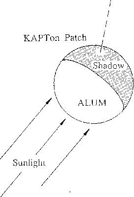
| Figure 1. Schematic showing the geometry used by EQUIPOT |
| Table of Contents | ECSS | Model Page |
| Background Information | Spacecraft charging | |
| Spacecraft charging: EQUIPOT | ||
Codes such as NASCAP are out of the scope of SPENVIS. Instead, the much simpler programme EQUIPOT, a part of the program suite ESPIRE, is implemented in SPENVIS. EQUIPOT sets out to do a similar job to MATCHG. It was developed in an attempt to model charging features observed on the Meteosat-2 spacecraft [Wrenn and Johnstone, 1987], using the measured electron flux spectra. EQUIPOT uses simple numerical integration of the multi-point spectra and voltage stepping to minimise net current, instead of seeking a time-based solution in terms of Maxwellian distributions. On realisation that it could also satisfy the ESA requirement for an engineering tool, it has been extended to address Low Earth Orbit environments, to enable the input of Maxwellian distributions and to include the effects of spacecraft velocity.
EQUIPOT Has been designed for a rapid assessment of the likelihood of charging for surface materials on a spacecraft. It utilises a simple geometry (a small isolated patch of material on a spherical spacecraft) to calculate the various components of current to both the body (structure) and the patch, and estimates the equilibrium potentials which will develop in order to achieve zero net current. Approximate charging time is also computed. The structure and patch materials are specified by the user, as well as the plasma environment by defining energy spectra for electron and ion fluxes, and/or Maxwellian distributions.
A number of options are available to cater for plasma regimes with Debye length large (GEO) or small (LEO), solar illumination or shadow, spacecraft velocity (ram and wake effects), and normal or isotropic incidence of particles. For small Debye length, it is reasonable to assume that current collection is sheath limited (plane probe assumption); for large Debye length, the geometry becomes important and a spherical probe assumption offers an alternative limit.
Secondary emission yield is a function of the energy of an incoming particle. To describe the yield for a selected material, the report file produced by EQUIPOT contains tables of values for incident electrons, including backscattering, and protons with isotropic and normal distributions and energy between 10 eV and 5 MeV. The adopted models from Whipple (1981) are described below.
For the structure it is possible to impose a potential. In this case, no other parameters are required for the structure.
The isolated patch may be of insulating or conducting material. In the latter case, it is necessary to specify the properties (thickness, conductivity, relative permittivity) of an intermediate insulator.
A number of pre-defined environments, listed in Table 1, are available. Alternatively, the user can fully specify the environment by entering the thermal spectra parameters and/or values for the flux spectra.
| Description | Thermal electron spectra | Thermal ion spectra | Electron flux spectrum | Ion flux spectra | Reference |
|---|---|---|---|---|---|
| Low altitude environments | |||||
| IRI at solar minimum, in winter, at 800 km, plus 10 kR aurora | 1 | 3 | yes | 1 | |
| IRI at solar maximum, in summer, at 800 km, plus 10 kR aurora | 1 | 3 | yes | 1 | |
| Maxwellians for 1,000 km plus aurora | 1 | 3 | yes | 1 | |
| Auroral type spectra from DMSP | 1 | 1 | yes | 1 | |
| Cold Maxwellians for ram test | 1 | 1 | no | none | |
| Test spectra and Maxwellians | 3 | 3 | yes | 1 | |
| Cold Single Maxwellian and Fontheim electrons | 1 | 1 | yes | none | Fontheim et al., 1982 |
| High altitude environments | |||||
| ECSS worst case model (SCATHA) | 2 | 2 | no | none | Gussenhoven and Mullen, 1983 |
| NASA guidelines worst case | 2 | 2 | no | none | Mullen and Gussenhovenn, 1982 |
| NASA guidelines average GEO environment | 2 | 2 | no | none | Purvis et al., 1984 |
| Meteosat very disturbed | none | none | yes | 1 | Wrenn and Johnstone, 1987 |
| Meteosat very quiet | none | none | yes | 1 | Wrenn and Johnstone, 1987 |
The current density J is a function of V which is both non-linear and non-local. The surface potential creates a plasma sheath in which the charged particle populations are modified from their ambient state. Current collection is then a function of sheath geometry which depends on the potentials of surrounding surfaces. Realistic modelling clearly requires to be three dimensional and NASCAP attempts the taks. However, even with 1200 elements there are practical limitations on the accuracy of definition for complex spacecraft systems. It is impossible to properly represent small items (e.g. solar array interconnects) which could be critically important if they support high potentials.
The sheath dimension relates to the Debye length lambdaD
(m) of the plasma as
In GEO, lambdaD is typically tens of metres, much larger than the dimensions of the surface element or even the spacecraft. In LEO, lambdaD is typically a few millimetres, much smaller than the dimensions of a satellite.
EQUIPOT Makes no attempt to realistically model the geometry, it assumes a very simple model of an isolated patch of material on the surface of a spherical spacecraft (see Fig. 1). The situation of a shadowed patch on a sunlit satellite is the one most likely to produce severe differential charging. Figure 2 illustrates the forms of sheath geometry which will develop in thick sheath and thin sheath extremes. The current-voltage characteristic for the patch will depend upon possible sheath expansion, as covered by Langmuir probe theory (see Fig. 3).
|
| Figure 1. Schematic showing the geometry used by EQUIPOT |
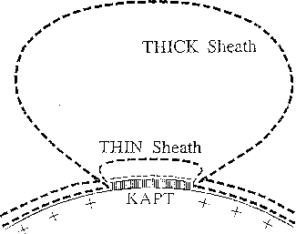 |
| Figure 2. Schematic of thick and thin sheath growth on an isolated patch |
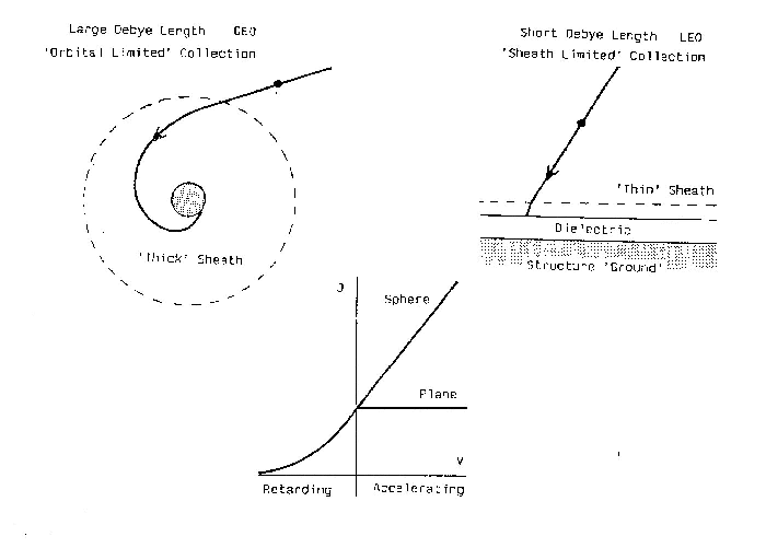 |
| Figure 3. Thick and thin sheath configurations with probe theory limits |
In the thin sheath limit (small lambdaD, LEO) the effective
collecting area cannot increase and the electron current is limited to the
random value pertaining to V=0:
The characteristics for ion current are the same but with a reversal of sign
for charge, V and J; however, Ji0 is much
smaller than Je0 because the random current is inversely
proportional to the square root of mass m. For a Maxwellian with temperature
T,
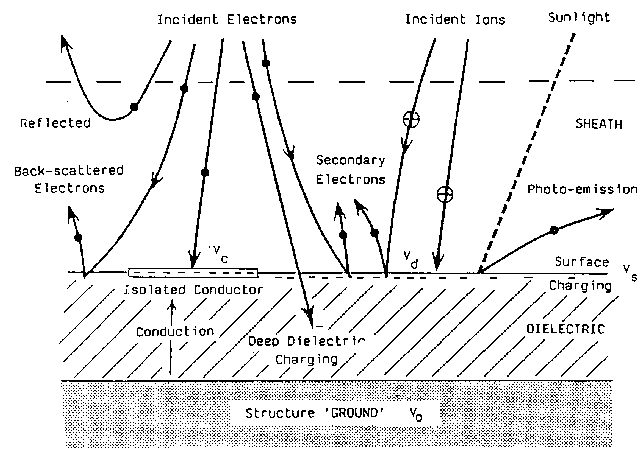 |
| Figure 4. Current components to a surface on a spacecraft |
For the numerical integration, the energy range of the input spectra is split
into intervals using linear interpolation. With flux spectra the energy
ranges are given by the limits of the input data. For Maxwellians, the minimum
and maximum energies are set to 0.05 kT and 10 kT,
respectively. Given a mixture of spectra and Maxwellians, the minimum and
maximum energies are the extremes from all components. In the latter case,
flux values are first taken from the input flux spectra and then from the
Maxwellians, outside the flux spectra ranges. The differential number flux for
a Maxwellian is given by
The electron and ion fluxes are converted to currents (nA m-2) by multiplication with the factor 109 pi e (e = 1.602x10⁻¹⁹ C). The secondary currents are then determined and all these components are integrated using a simple Simpson rule procedure. Given a surface potential V, the integration is cut off below energies eV for retarded particles.
If the surface is positive, not all photo-electrons and secondary electrons will escape. The corresponding currents are then reduced by a factor exp(-0.5 V/Ts), where Ts is the effective temperature of the emitted electrons. Following Whipple [1981], the temperatures are specified as follows:
| photo-electrons: | 3 eV; |
| secondaries from electrons: | 2 eV; |
| secondaries from protons: | 5 eV. |
| Jbe = Yb Je |
| Jsi = Ysi Ji |
| Jse = Yse Je |
for either normal or isotropic incidence of the input fluxes.
| Es (eV) | Yb |
|---|---|
| >100,000 | 0 |
| 10,000-100,000 | 1 - 0.73580.037Z |
| 1,000-10,000 | 1 - 0.73580.037Z + 0.1 exp(-Es/5,000) |
| 50-1,000 | 0.3338 ln(Es/50) [1 - 0.73580.037Z + 0.1 exp(-Es/5,000)] |
| <50 | 0 |
where Z is the atomic number. For isotropic incidence, the normal value Yb is transformed to 2 (1-Yb+YblnYb) / ln2Yb.
     Q = 0             for         Es > 10
     Q = 1/Es - 0.1    for 0.476 < Es < 10
     Q = 2             for         Es < 0.476
The accuracy of secondary electron yields is crucial to charging analysis (Katz et al., 1986). Therefore, four different formulations of the emission yield are implemented in EQUIPOT.
For isotropic incidence,
First a maximum range Ru is calculated, i.e.
R=Ru when
Yield as a function of directional flux, with angle of incidence
theta, is given by:
In the event that the full set of range parameters for the Katz formula
are not available, then a formula by [Feldman, 1960] may be used
to infer them from the density rho, the atomic number A
and the mean molecular weight mu:
    n1 = 1.2 / [1 - 0.29 log(A)]
    R1 = 250 mu / rho * A-0.5n1
    n2 = 0
    R2 = 0
The use of this
approximation has been implemented in order to be complementary with
NASCAP and MATCHG.
The additional root-finding and numerical fitting involved in the Katz algorithm and, to a lesser extent the Sims algorithm, makes the code potentially less stable than with the Whipple formula alone. This is because bad values input by users may result in situations where there is no sensible root or fitted value. The code will capture two cases:
The code employs a potential stepping algorithm, controlling direction and increment, to minimise Jnet and locate equilibirum assuming a single root solution (see Fig. 5 for a flow chart of the algorithm). The voltage step is repeatedly multiplied by a factor of ten until Jnet changes sign. When this occurs, the voltage step is reduced by a factor of ten, a new loop is initiated and continued with further reductions until equilibrium is reached (i.e. the voltage step is reduced to less than either 0.001 V or 0.02 V).
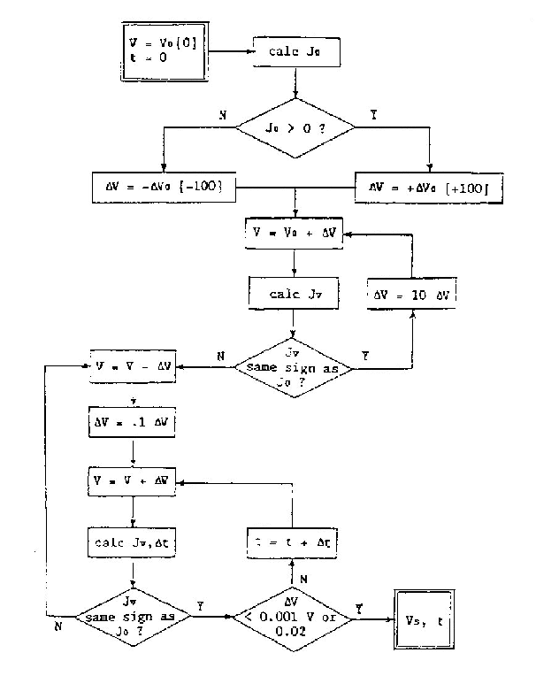 |
| Figure 5. Voltage stepping algorithm used by EQUIPOT |
The charging time is estimated by determining
Delta t = CA Delta V / Jmean
for each step and
summing over all steps to equilibrium. Here Jmean is the mean
current during the step and CA is the capacitance per unit
area. Of course, the error in Delta t relates directly to the size of
Delta V since constancy of Jnet through the step is
assumed. An equivalent charging time constant T is determined at the
final step as
RAM_OFF, RAM_ON, or WAKE_ON.
In the RAM_ON configuration, thermal ion components with
temperatures less than 5 eV are treated as drifting Maxwellians. The integrated
current densities are then given by:
In the WAKE_ON configuration, a wake void is assumed such that the
thermal ion current to the patch is further reduced by a factor of sine(angle
of attack > 90°).
The user is probably concerned with worst case situations and EQUIPOT is an excellent tool for identifying these. Following a realistic scan of all the variables and finding no equilibrium potential above 100 V, the user can be confident that there is no serious charging problem. On the other hand, potentials above 1000 V would certainly justify a more detailed study. Results between 100 V and 1000 V should prompt the user to seek parameter changes which would reduce the predicted charging to an acceptable level; expedient design modification may then be indicated.
Feldman, C., Phys. Rev., 117, 455, 1960.
Fontheim, E. G.,Statistical Study of Precipitating Electrons, Journal of Geophysical Research, VoL 87, No. A5, p. 3469-3480, 1982.
Gussenhoven, M. S., and E. G. Mullen, Geosynchronous Environment for Severe Spacecraft Charging, J. Spacecraft and Rockets, 20, 26, 1983.
Katz, I., et al., A three-dimensional study of electrostatic charging in materials, NASA CR-135256, 1977.
Katz, I., M. Mandell, G. Jongeward, and M. S. Gussenhoven, The importance of accurate secondary electron yields in modeling spacecraft charging, J. Geophys. Res., 91, 13,739-13,744, 1986.
Martin, A. R., et al., Large Polar Orbiting Spacecraft Plasma Wake Studies, Final Report on MOD(PE) Contract SLS32A/1937, 1990.
Gussenhoven, M. S., and E. G. Mullen, A "Worst Case" Spacecraft Environment as Observed by SCATHA on 24 April 1979, AIAA Paper 82-0271, Jan. 1982.
Purvis, C. K., H. B. Garrett, A. C. Whittlesey, and N. J. Stevens, Design Guidelines for Assessing and Controlling Spacecraft Charging Effects, NASA Technical Paper 2361, 1984.
Sims, A.J., Electrostatic Charging of Spacecraft in Geosynchronous Orbit, Tech Memo SPACE, 389, DRA 1992.
Whipple, E. C., Potentials of surfaces in space, Rep. Prog. Phys., 44, 1197-1250, 1981.
Wrenn, G. L., Spacecraft Charging Effects, RAE Tech Memo SPACE 375, 1990.
Wrenn, G. L., and A. D. Johnstone, Evidence for Differential Charging on Meteosat-2, J. Electrostatics, 20, 59-84, 1987.
Wrenn, G. L., and A. J. Sims, The 'Equipot' Charging Code, Working Paper SP-90-WP-37, 1990; updated by D.J. Rodgers, 2002.