Help: Single event upsets

Table of Contents	ECSS	Model Page
Background Information	Background Information
	Single event upsets

Overview

Single event upsets (SEUs) occur when a single ionising radiation event produces a burst of hole-electron pairs in a digital microelectronic circuit that is large enough to cause the circuit to change state. In space, these unplanned changes of state usually result from the direct ionisation of single heavy ions originating outside the spacecraft, or by the products of nuclear reactions initiated by particles that originated outside the spacecraft. The Cosmic Ray Effects on MicroElectronics (CREME) model suite (Adams, 1986) was developed by the Naval Research Laboratory (NRL) to assess the SEU rates in the radiation environments that can be expected during space missions. CREME Provides models for the following quantities:

the near-Earth particle environment outside the magnetosphere;
the orbit-averaged geomagnetic cutoff transmission function that is used to modulate the environment outside the magnetosphere to any spacecraft orbit;
transportation of the radiation environment through the walls of the spacecraft;
transformation from energy spectra to Linear Energy Transfer (LET) spectra;
computation of SEU rates caused by direct ionisation and by proton-induced nuclear reactions.

The near-Earth particle environment

Geomagnetic cutoff effects

The ability of charged particle radiation to penetrate into the magnetosphere from outside is limited by the Earth's magnetic field. The number of magnetic field lines a cosmic ray must cross to reach a given point within the magnetosphere approximately determines the minimum energy it must possess. To cross more magnetic field lines more energy will be required. A particle's penetrating ability is determined uniquely by its momentum divided by its charge, a quantity called magnetic rigidity.

Particles having low magnetic rigidity (i.e. momentum per unit charge) are preferentially turned back by the field, so they are unable to penetrate beyond some depth in the magnetosphere. For each point in the magnetosphere and for each direction of approach to that point, there exists a threshold value of magnetic rigidity, called the geomagnetic cutoff. Below this value, no charged particle can reach the specified point from the specified direction. Above this cutoff value, particles arrive at the specified point from the specified direction as though the magnetic field were not present at all (Lemaître and Vallarta, 1933). Regions in the outer magnetosphere and near the poles can be reached at much lower magnetic rigidities than are required to reach points near the Earth's equator.

Computation of the cutoff

The geomagnetic cutoff was first calculated by C. Störmer (1930), using a dipole approximation for the Earth's magnetic field:

P_c = 59.6 r^-2 [1-(1-cos gamma cos³ lambda)^1/2]² (cos gamma cos lambda)^-2
for positively charged particles, where P_c is the magnetic rigidity in GeV/ec, r the radial distance from the dipole centre in Earth radii, lambda the latitude in eccentric dipole coordinates, and gamma the arrival direction measured from magnetic west.

The magnetic rigidity is related to the particle's energy by:

E = (M₀² + P²Z²/A²)^1/2 - M₀ ,
where E is the kinetic energy in GeV/u, A is the particle's mass in amu, Z is the particle's charge, and M₀=0.931 GeV. P_c Strongly depends on the geomagnetic latitude, which means that the geomagnetic cutoff varies drastically around the orbit of a spacecraft, especially at high inclinations.

As the geomagnetic cutoff varies with the particle's arrival direction, the geomagnetic cutoff transmission has to be averaged over all arrival directions. In the SPENVIS implementation of CREME, this is achieved by a numerical integration over the arrival direction. This is done for each point on the spacecraft orbit, and for each particle energy and charge. SPENVIS also allow to set a vertical cutoff as an effective average over arrival directions, which is described by the CREME formula P_c = 16/L² or its update (see Tylka et al., 1997) P_c = 14.5/L². Above L=5 no shielding is assumed.

Effects of the Earth's shadow

Störmer's theory does not account for the presence of the solid Earth, so in some directions at each location, this theory predicts a cutoff that is lower than the actual cutoff. The problem of the Earth's shadow was first addressed by Vallarta (1948), again in the context of the dipole model. Vallarta showed that there existed a range of magnetic rigidities above the Störmer cutoff where the Earth's shadow casts a broken pattern of allowed and forbidden bands of magnetic rigidity. The width of the penumbral shadow of the Earth varies from 10/ to 100/ above the Störmer cutoff at the Earth's surface for zenith angles <45°. For larger zenith angles, the effect increases as the arrival direction approaches the horizon. The density of the penumbral shadow is also highly variable.

On the Earth's surface the effect of the Earth's shadow is simple: particles can arrive from above, not below. For high energies, the portion of the geometry factor that is occulted falls off with altitude h as:

Omega = 2pi {1 - [(R_E+h)² - R_E²]^1/2 / (R_E+h)} .
At lower magnetic rigidities, the Earth's umbral shadow is distorted by the Earth's field and swept off to an easterly direction so that particles may arrive below the optical horizon in the west. This distortion increases at lower rigidities as the cutoff is approached. Besides the change of direction of Earth occultation at low rigidities, the occulting solid angle also falls off more rapidly with altitude than described by the equation above (Smart, 1980). The details of how the Earth's umbral shadow changes with altitude and rigidity are unknown. Smart (1980) has suggested that the problem might be solved by ray tracing at a range of altitudes and rigidities.

Effects of geomagnetic storms

The discussion above supposes a quiescent magnetosphere. When a solar flare occurs, it usually causes a magnetic storm at the Earth. These storms disrupt the magnetosphere altering the geomagnetic cutoff, usually depressing it. The effect seems to be the result of ring currents induced by the sudden commencement of the storm (Fluckiger et al., 1979; Dorman, 1974). These currents reduce the equatorial magnetic field by about 0.01 gauss, allowing penetration to any given point in the magnetosphere by lower energy cosmic rays than is normally possible.

The effect of geomagnetic storms can be modelled as follows:

P_storm = P_c [1 - 0.54 exp(-P_c/2.9)] .
Obviously, the actual degree of supression will vary from one magnetic storm to another, and the above expression only provides an average correction.

Radiation transport through the walls of the spacecraft

Once the differential energy spectrum of each element at the skin of the spacecraft has been determined by modulating the near-Earth and trapped radiation environments with the geomagnetic cutoff transmission function, a transport calculation must be performed to find the differential energy spectra at the microelectronic components inside the spacecraft. CREME Takes into account the effects of energy loss and particle losses through total inelastic collisions (Adams, 1983). No account is taken of the way in which the projectile fragments from these collisions contribute to the differential energy spectra of lighter ions. This omission results in a systematic underestimate of the particle fluxes, especially for the elements from argon through manganese. This underestimate is so small that it can be neglected for shielding thicknesses typically found in spacecraft.

The differential energy spectrum f(E) inside the spacecraft and behind a thickness t (in g cm^-2 of Al or equivalent) of shielding, is given by:

f(E) = f'(E') [S(E')/S(E)] exp(-sigma t) ,
where
sigma = [5x10^-26 eta (A^1/3+27^1/3-0.4)²] / 27 ,
f'(E') is the differential energy spectrum at the skin of the spacecraft, E' is the energy at the skin of the spacecraft (E'=R^-1 [R(E)+t], where R(E) is the residual range of an ion having an energy E and R^-1 is the inverse function of R(E)), E is the energy inside the spacecraft, S(E) is the stopping power of an ion with energy E, A is the atomic mass of the ion, and eta is Avogadro's number.

Range-energy and stopping power data are provided by Adams et al. (1987). The differential energy spectra inside spacecraft estimates by the equations above are satisfactory for estimating SEU rates provided the shielding thickness does not exceed 50 g cm^-2. For greater shielding thicknesses, this method seriously underestimates the SEU rate (Adams, 1983). Precise estimates can be made by an exact transport calculation, following the methods of Tsao et al. (1984).

Calculation of the LET spectrum

The next step is to calculate the Linear Energy Transfer (LET) spectrum from the differential energy spectra at the microelectronic components inside the spacecraft. LET Is the rate at which energy is deposited per unit path length of an ionising particle. For the present purpose, it is equivalent to the rate of energy loss per unit path length for the same particle, i.e. dE/dx or stopping power.

The transformation from a differential energy spectrum to a differential LET spectrum is

f(S) = f(E) dE/dS .
This equation has singularities at the points where dS/dE becomes zero. In the computer programme the ratio of finite differentials is used to approximate dE/dS and if the boundaries of the intervals in E and S are properly chosen, the ratio can be kept finite. Even then, spikes appear in the differential LET spectra, which makes them hard to handle on a computer. Instead, integral LET spectra are used.

The final step is to repeat the calculation of f(S) to the differential energy spectra for all the elements in cosmic rays (i.e. protons to uranium) and sum the resulting integral LET spectra to form one composite integral LET spectrum. This spectrum can then be used to estimate SEU rates that result from the direct ionisation of charged particles.

Calculation of SEU rates from the direct ionisation of charged particles

An SEU occurs when a sufficiently large burst of charge is collected on a critical node in one of the digital microcircuits on a chip. The minimum charge required to produce an SEU is called the critical charge. This burst of charge can come from a segment of the ionised trail left by the passage of an intensely ionising particle. It is assumed that each critical node is surrounded by a sensitive volume (idealised as a rectangular parallellopiped = RPP model) and that the charge deposited in this volume is collected (Pickel and Blandford, 1980). The dimensions of the sensitive volume are related to those of the critical node. The sensitive volume is not, however, just the dimensions of this feature. Charge is also collected by diffusion from the material surrounding the node. The efficiency of charge collection from beyond the node falls off with distance. Pickel and Blandford (1980) discuss how the critical charge and the dimensions of the sensitive volume are found. In general, experimental measurements of the operational SEU cross section for the device, as well as design data supplied by the manufacturer, are required. It is often necessary to interpret these data using detailed circuit modelling software before the device SEU parameters can be determined.

The simple model described above predicts that when the critical charge has been collected, an SEU will occur. The amount of charge collected depends linearly on the LET of the ionising particle and the length of its path withing the sensitive volume. There is, however, another effect that extends the size of the sensitive volume. The intense trail of ionisation left by the charged particle alters the electric field pattern in the neighbourhood of the feature. The field forms a funnel along the particle track and this enhances the efficiency with which charge is collected. This funnel effect can be partly accounted for in the simple model discussed above if the dimensions of the sensitive volume are experimentally determined.

For estimating the soft upset rates due to the direct ionisation by particles originating outside the spacecraft two methods are implemented in SPENVIS: the rectangular parallellopiped (RPP) and the integral rectangular parallellopiped (IRPP) method. Which one is applied, depends on the cross-section method i.e. RPP when the critical charge is given and IRPP when the cross sections are provided by a Weibull function or a table. We describe both methods briefly.

In the RPP method it is assumed that above a unique critical charge Q_c all bits of equal size, are upset. In this idealized situation the upset cross section curve is presented as a step function, equal to zero below some threshold value of the LET and equal to a constant value above it (see figure 1 dashed line). The upset rate U (in bit^-1 s^-1) has been described by Adams (1983) and is given by:

expression 1 for direct ionisation upset rate

where A is the surface area of the sensitive volume in m², (X/e) the ratio of the energy X that is needed to create one electron-hole pair (3.6 eV in Si; 4.8 eV in GaAs) to the elementary charge e (= 1.602·10^-19C) that converts pC to MeV, Q_c the minimum charge in pC required to produce an upset, L_min=(X/e)·Q_c/p_max the required minimum LET in MeV·cm²·g^-1 for an upset with p_max the largest diameter of the sensitive volume in g·cm^-2, L_max=1.05x10⁵ MeV·cm^2·g^-1 the highest LET any stopping ion can deliver, L the LET in MeV·cm²·g^-1, F(L) the integral LET spectrum in particles·m^-2·s^-1·sr^-1 and D[p(L)] the differential path length distribution in the sensitive volume of each memory cell in cm²· g^-1 with p(L)=(X/e)·Q_c/L the path length over which an ion of LET L will produce a charge Q_c.

The equation for U contains the implicit assumption that the LET of each ion is essentially constant over the dimensions of the critical volume. Of course, this is not true for stopping ions very near the end of their range. The equation assumes that the maximum LET of the stopping ion applies over its entire path length in the sensitive volume. This assumption can result in calculated energy depositions that exceed the residual energy of the ion. The problem is especially acute for large sensitive volume dimensions and threshold LET values just below the maximum LET of an ion that is much more abundant than all heavier ions. Fortunately, this circumstance rarely arises. The equation for Uis accurate if the flux of stopping ions is small compared to fast ions having the same LET. Care should be taken in the use of this formula when the threshold LET is just below the edge of a "cliff" in the integral LET spectrum.
Furthermore, the equation for U assumes one continuously sensitive critical node per bit. In general, there may be several critical nodes per bit, each with its own sensitive volume dimensions and critical charge. In addition, these nodes may only be sensitive part of the time, making it necessary to calculate partial upset rates for each node and then combine the results, weighted by the fractional lifetime of each node.

When using the RPP method to user has to enter the critical charge Q_c in pC.

More accurate estimations of the upset rate can be made using the experimental cross section curve which shows a more gradually increase to a saturated cross section, σ_lim, instead of the sharp cut-on adopted in the RPP method (see figure 1 full line). In this case the upset rate is given by the sum of a step-wise set of differential upset-rate calculations and is called the IRPP method (Petersen, 1997):

expression 2 for direct ionisation upset rate

where each U_i is calculated with the RPP method whereby using σ_i and L_i respectively as surface area and minimum LET. The cross sections σ_i are either given in a table of cross sections (cm²/bit) vs. LET (MeV⋅cm²/mg) values or described by a four-parameter Weibull fit.

Default devices are the silicon 93L422AM device (Petersen, 1998) with a Weibull fit as cross section method and the gallium-arsenide MESFET 1K SRAM device (Weatherford et al., 1991) with a critical charge as input.

Figure 1. Idealised (dashed line) and representative cross section curves (full line).

Improved algorithms

The CREME method with constant LET treatment has two major flaws which are summarized as:

1) The maximum LET of the stopping ion is applied over its entire path length in the sensitive volume which may result in calculated energy depositions that exceed the residual energy of the ion and thus overestimates the upset rate.
2) Ions with an energy below the minimum energy for an upset may still produce an upset as long as the deposit energy (E_dep=L⋅p) is larger than the minimum energy.

To meet the first shortcoming an improved algorithm has been implemented that accounts for the variation of the LET inside the volume. In the approach the required minimum path length p_min for depositing the minimum energy E_min for an upset is obtained from the condition:

with ΔE the energy loss after crossing a distance p. The energy loss is computed from the LET curve as function of energy and averaged over all species envolved i.e.:

with F(E_i) and L(E_i) respectively the energy flux and LET curve for species i with energy E.

To account for the fact that ions with the same LET value have different energies, we implemented the "slowing and stopping ion" algorithm that uses the ion energy spectra instead of the LET spectrum to calculate the upset rates by direct ionisation. In this way only ions with an energy above the minimum energy can cause an upset. Using the differential ion energy spectra as input, the upset rate is given by,

with F(E,Z) the differential ion energy flux in #⋅m^-2⋅ s^-1⋅sr^-1⋅MeV^-1. When the ion stops inside the volume i.e. E(initial) - E(after crossing path length p) < 0, the deposit energy is equal to E(initial). The maximum energy E_max corresponds with the maximum energy in the spectrum.

Calculation of SEUs resulting from nuclear reactions caused by protons

For proton irradiation only a very few sensitive devices are affected by direct ionization-induced charge but nuclear reactions within shielding material can produce recoil particles with high enough LET to cause effects. An estimate of the upset rate from nuclear interactions of energetic protons can be obtained by integration of the product of the measured proton-induced upset cross section σ(E) and the differential proton flux f(E) inside the spacecraft, over all energies:

expression 2 for direct ionisation upset rate

with U in bit^-1·s^-1 and f(E) in protons·m^-2· s^-1·sr^-1·MeV^-1.

If experimental values for σ(E) are available they can be entered in a table of cross section (cm²/bit vs. energy (MeV) values which are then either fitted to a 2-parameter Bendel or a 4-parameter Weibull function or are linearly interpolated. In case no fit is required the user can just enter the Bendel or Weibull function parameter values.

The 2-parameter Bendel function is given by (e.g. Stapor et al., 1990):

with

where E and A are in MeV and 'A' corresponds to an energy threshold for upset and is fitted to experimental data (at or near 60 MeV). Sometimes σ_lim is written as (B/A)¹⁴ where B is the second Bendel parameter.

The 4-parameter Weibull function is given by (e.g. Petersen, 1992):

with E₀ the threshold or onset energy in MeV, σ_lim the saturation cross section in cm²·bit^-1, W the width of the rising portion of the curve in MeV and S the power that determines the shape of the curve.

For the default silicon device 93L422AM (Tylka et al., 1996) a Bendel fit is used while for the gallium-arsenide MESFET 1K SRAM device (Weatherford et al., 1991). experimental data are implemented and linearly interpolated

When no experimental data are avalaible, the PROFIT or SIMPA method can be used to calculate the proton-induced upset cross-sections on basis of heavy ion-induced cross-section data.

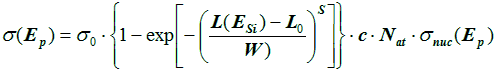
PROFIT method (Calvel et al., 1996):

with

σ₀, L₀, W and S the Weibull fit parameters
E_p, the incident proton energy
E_Si, the energy of the Si recoil ion after elastic nuclear scattering at an average diffusion angle T of protons
L(E_Si),the electronic stopping power for Si ion in Si
N_at, the number of Si atoms per cm³
σ_nuc, the elastic cross section in cm² for proton-Si nuclear reactions
c, the depletion depth

The PROFIT method is also available for gallium-arsenide devices.

SIMPA method (Doucin et al., 1994): (not yet available)

with

E_p, the incident proton energy
E_s, the energy deposited by the secondary recoils
σ_hi, the heavy ion cross section
Φ(E,E_p), the propability that a recoil Si ion of energy E is generated by an incident proton of energy E_p.

For the heavy ion cross section a Weibull fit is adopted.

The proton differential energy spectra can be obtained with the trapped proton models implemented in SPENVIS and with the exomagnetospheric proton models (both for cosmic rays and solar flares) that are implemented in SPENVIS (the exomagnetospheric components have to be modulated to the spacecraft orbit). The combined proton differential energy spectrum incident on the skin of the spacecraft can then be propagated to the electronics inside using a simplified version of the equation given above for the differential energy spectrum inside the spacecraft .

References

Adams, J. H., Jr., The Variability of Single Event Upset Rates in the Natural Environment, IEEE Trans. Nucl. Sci., 30, 4475-4480, 1983.

Adams, J. H., Jr., Cosmic Ray Effects on MicroElectronics, Part IV, NRL Memorandum Report 5901, 1986.

Adams, J. H., Jr., J. Bellingham, and P. E. Graney, A Comprehensive Table of Ion Stopping Powers and Ranges, NRL Memorandum Report, 1987.

Adams, J. H., Jr., J. R. Letaw, and D. F. Smart, Cosmic Ray Effects on MicroElectronics, Part II: The geomagnetic cutoff effects, NRL Memorandum Report 5099, 1983.

Bendel, W. L., and E. L. Petersen, Proton Upsets in Orbit, IEEE Trans. Nucl. Sci, NS-30, 4481-4485, 1983.

Calvel, P., Barillot, C., Lamothe, P., An Empirical Model for Predicting Proton Induced Upset, IEEE Trans. On Nucl. Science , Vol. 43, No. 6, 1996.

Doucin, B., Patin, Y., Lochard, J.P. et al., Characterization of proton interactions in electronic components, IEEE Trans Nuc Science, Volume 41, Issue 3, Jun 1994 Page(s):593 � 600.

Lemaître, G., and M. S. Vallarta, Phys. Rev., 43, 87, 1933.

Petersen, E.L., Pickel, J.C., Adams, J.H., Jr. and Smith, E.C., Jr., Rate Prediction for Single Event Effects--A Critique, IEEE Transactions on Nuclear Science , NS-39, Dec 1992, pp 1577-99

Petersen, E.L., Single-event analysis and prediction, Short Course Notes, ch. III, IEEE Nuclear and Space Radiation Effects Conference, Snowmass, 21 July 1997.

Petersen, E.L., The SEU figure of merit and proton upset rate calculations, Nuclear Science, IEEE Transactions on Volume 45, Issue 6, Dec 1998 Page(s):2550 - 2562

Pickel, J. C., and Blandford, J. T., Jr., Cosmic-Ray-Induced Errors in MOS Devices, IEEE Trans. Nucl. Sci., NS-27, 1006-1015, 1980.

Stapor, W.J., Meyers, J.P., Langworthy, J.B., Petersen, E.L., Two parameter Bendel model calculations for predicting protoninduced upset [ICs], Nuclear Science, IEEE Transactions on Volume 37, Issue 6, Dec 1990 Page(s):1966 - 1973

Størmer, C., Periodische Elektronenbahnen im Felde eines Elementarmagneten und ihre Anwendung auf Br�ches Modellversuche und auf Eschenhagens Elementarwellen des Erdmagnetismus. Mit 32 Abbildungen., Zeitschrift für Astrophysik, Vol. 1, p.237, 1930.

Tsao, C. H., Silberberg, R., Adams, J. H., Jr. and Letaw, J. R., Cosmic Ray Effects on MicroElectronics, Part III: Propagation of Cosmic Rays in the Atmosphere, NRL Memorandum Report 5402, 1984.

Tylka, A.J., Dietrich, W.F., Boberg, P.R., Smith, E.C.and Adams, J.H., Jr., Single event upsets caused by solar energetic heavy ionsNuclear Science, IEEE Transactions on Volume 43, Issue 6, Dec 1996 Page(s):2758 - 2766

Tylka, A.J. et al.,"CREME96: A Revision of the Cosmic Ray Effects on Micro-Electronics Code", IEEE Transactions on Nuclear Science, 44, 2150-1260 (1997).

Vallarta, M.S., On the Energy of Cosmic Radiation Allowed by the Earth's Magnetic Field, Phys. Rev. 74, 1837�1840 (1948)

Weatherford, T.R., Petersen, E., Abdel-Kader, W.G., McNulty, P.J., Tran, L., Langworthy, J.B. and Stapor, W.J., Proton and Heavy Ion Upsets in GaAs MESFET Devices, IEEE Trans. Nucl. Sci. NS-38, 1450 - 1456 (1991).

This description is mainly based on the report of Adams (1986).

Last update: Mon, 12 Mar 2018